Modifying Custom Matmul CUDA Kernels
I started to learn CUDA last year, and started writing matrix multiplication kernels as a learning project. After some struggles, I made them to work, but then got disappointed when I saw my kernels are 10 times slower than cuBLAS GEMM kernels. Maybe my expectations were a bit too high. I’ve tried lots of open sourced matmul kernels on github, but the best one I found was still about 5 times slower (some of them were optimized for older architectures). So I started the journey of optimizing my own matmul kernel. After few months of trial and error, my matmul kernel finally has comparable speed to cuBLAS GEMM.
Why would you need to write your own matmul kernel? the answer is, in most cases you don’t need to and also shouldn’t. It simply isn’t worth the effort when there are highly optimized cuBLAS kernels available.
There are two reasons why I did it:
- It’s a great project to learn about CUDA programming and GPU architectures.
- It’s the only way if you want to customize / modify matrix multiplcation, because cuBLAS is not open sourced.
In this post, I mainly want to talk about the second point: some modifications that can be done on matmul kernels and their applications.
Note: all of the kernel optimizations are targeted towards devices with compute capability 7.5 (Tesla T4, RTX 20 series), all experiments are done with a Tesla T4 GPU on Google Colab. Performance on other GPUs may not be optimal.
Note: all source code can be found in this repository.
Table of contents:
Batch Matrix Multiplication (BMM)
BMM is basically multiplying a batch of (M x K) matrices with a batch of (K x N) matrices, and get a batch of (M x N) matrices as a result. When batch size is equal to 1, it becomes a regular matrix multiplication. here is an example code in pytorch:
a = torch.randn(batch_size, M, K)
b = torch.randn(batch_size, K, N)
c = torch.bmm(a, b)
# c has shape [batch_size, M, N]
Here is the source code of my BMM kernel.
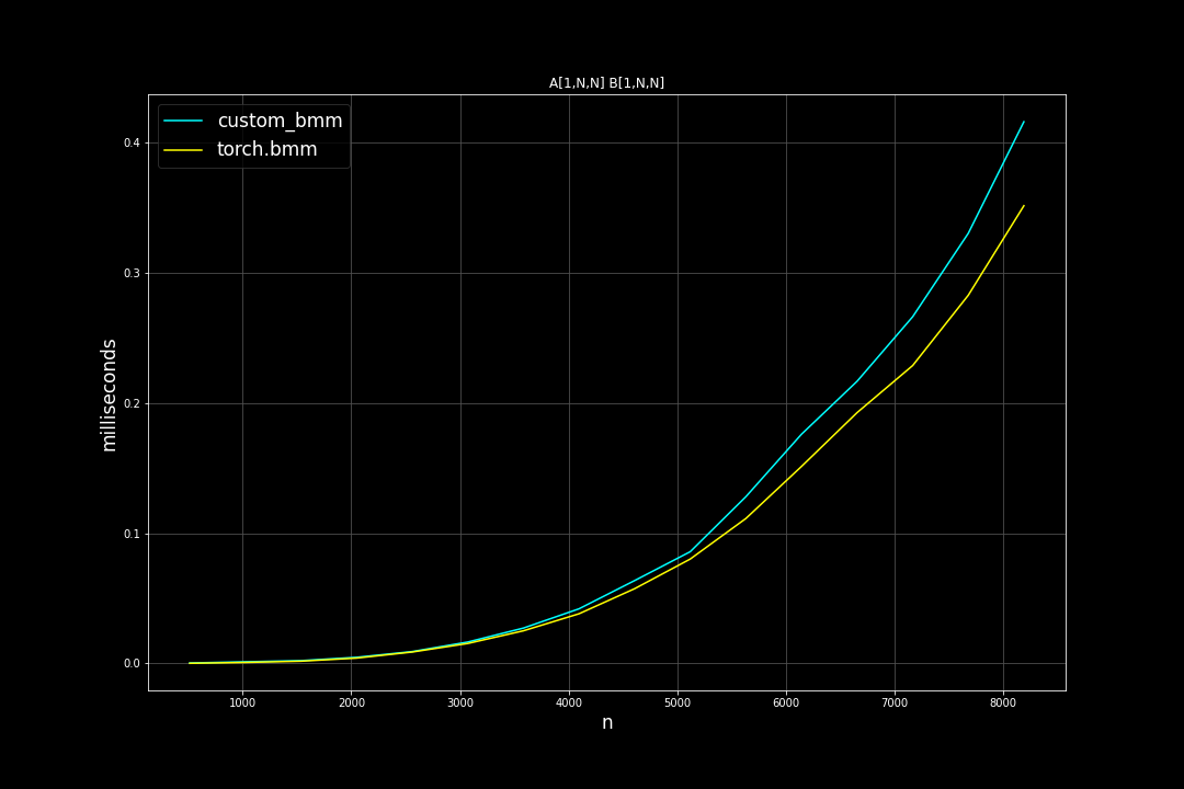
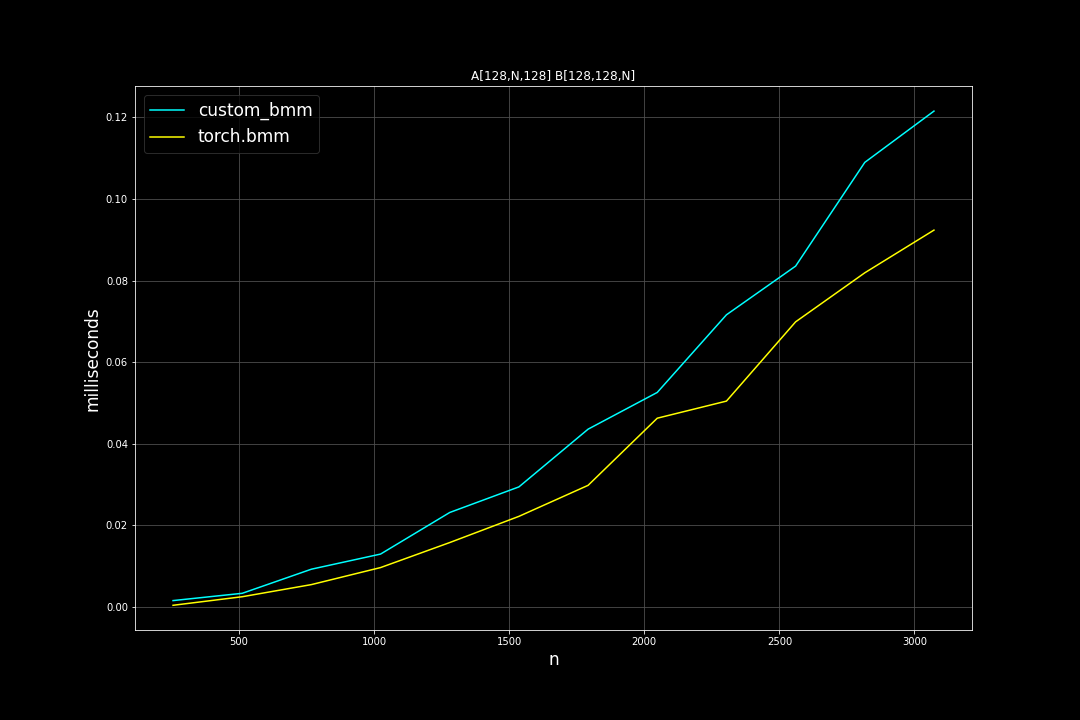
Here are some speed comparisons between my BMM kernel and torch.bmm which calls cuBLAS GEMM.
Click here to show plots
Square matrices: batch size = 1, varying M, N, K (M = N = K)
Runtime (ms):
Batch size = 128, K = 128, varying M, N (M = N)
Runtime (ms):
Fused Reduce Matmul
Sometimes we want to apply reduction right after a matrix multiplication:
c = torch.bmm(a, b)
max_c, argmax_c = torch.max(c, dim=1)
sum_c = torch.sum(c, dim=2)
argmin_c = torch.argmin(c, dim=1)
Normally there isn’t a problem with doing this, however, when I was implementing k-means clustering for TorchPQ, this became an issue. One of the major steps of k-means clustering algorithm is the computations of pairwise distance between all data points and all centroids (cluster centers), then getting the index of the closest cluster for each data point (argmin).
When the number of data points (n_data) and the number of clusters (n_clusters) are very large, this step will produce a huge (n_data x n_clusters) matrix that might not fit into the GPU memory (imagine a 1,000,000 x 10,000 fp32 matrix)
One workaround is to split this step into multiple tiny steps: in each step only compute the distance between a subset of data points and centroids (let’s say 10,000 x 10,000), then asign each data point in the subset to the closest cluster, and repeat.
A better solution could be to fuse argmin into the matmul kernel. Advantages of doing this are:
- No need to create a huge pairwise distance (or dot product) matrix if the result of argmin (or any type of reduction) is all we care about.
- Possibily faster because of fewer memory loads. Global memory loads and stores are usually one of the major bottlenecks of CUDA kernel optimization. When calculating pariwise distance / dot product, kernels will store results back to global memory at the end of calculation, another reduction kernel will have to load values from the same global memory location, then perform the reduction. By fusing reduction into the matmul kernel, we will skip the global memory read step.
I will not go into details in this post, if you are interested, you can read implementation details, and check the source code.
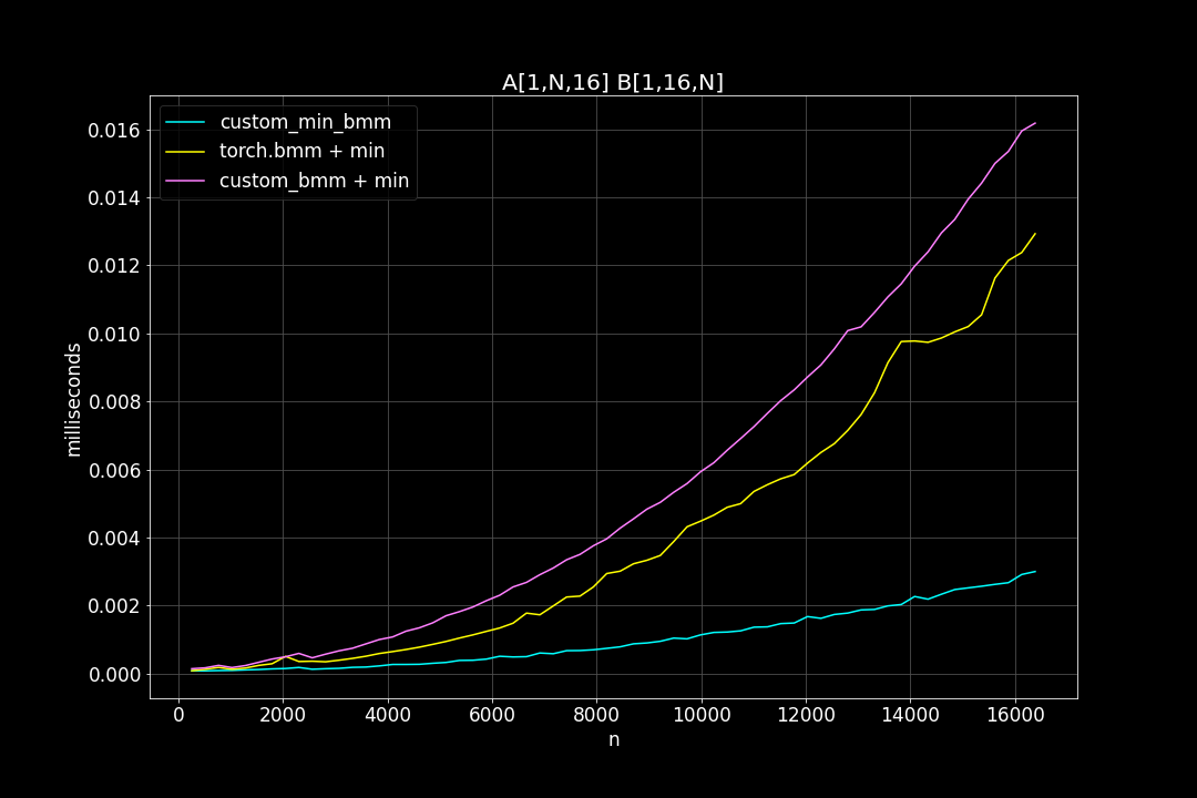
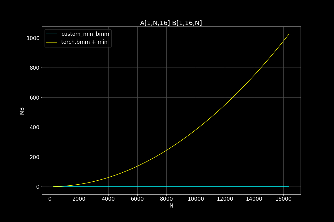
I compared the new MinBMM kernel with 2 things:
values, indices = torch.min( torch.bmm(a, b), dim = dim)
and
values, indices = torch.min( custom_bmm(a, b), dim = dim)
And here are the results:
Click here to show plots
batch_size = 1, K = 16, varying M, N (M = N)
Runtime (ms)
Peak Memory Usage (MB)
batch_size = 1, K = 64, varying M, N (M = N)
Runtime (ms)
Peak Memory Usage (MB)

batch_size = 1, K = 256, varying M, N (M = N)
Runtime (ms)
Peak Memory Usage (MB)


batch_size = 64, K = 64, varying M, N (M = N)
Runtime (ms)
Peak Memory Usage (MB)
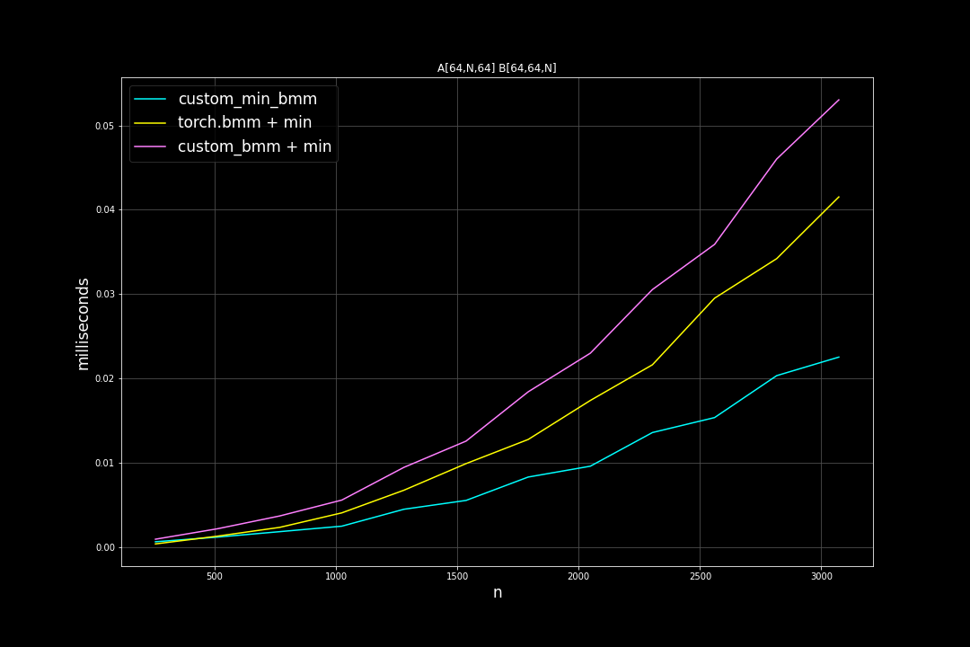
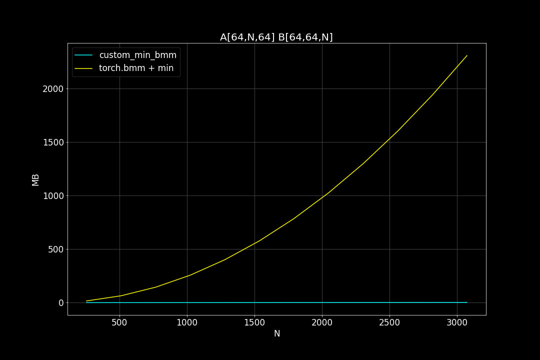
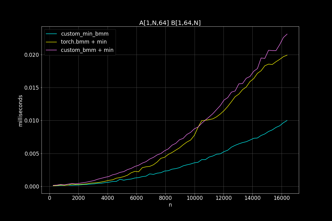
From the benchmark results we can see that fused MinBMM kernel is much faster than calling min and bmm kernels seperately, especially when k is smaller. The speedup seems to decay as K growth larger. Another advantage of MinBMM is the required memory is much smaller than other methods, the inputs can be (1,000,000 x K) matrices, and we still don’t need to be worried of going out of memory.
L2 distance
For L2 distance, all we need to change is a single line in thread_matmul:
cCache[m].val[n] = fmaf(a, b, cCache[m].val[n]);
to
float dif = a - b;
cCache[m].val[n] = fmaf(dif, dif, cCache[m].val[n]);
Now the BMM kernel will calculate squared L2 distance instead of dot product. We don’t calculate square root since it doesn’t affect the order of nearest neighbors.
Topk Search
Nearest Neighbor Search (NNS) and Maximum Inner Product Search (MIPS) are some of the most important components of information retrieval and data science. Sometimes it’s required to search in million or billions of vectors with thousands of queries within seconds.
The naive way is to calculate pairwise distance matrix (or dot product) of dataset vectors and query vectors first, then apply topk search after. This is also called “bruteforce search”. Here is an example in pytorch:
n_data = 1_000_000
n_query = 1000
d_vector = 256
a = torch.randn(n_data, d_vector)
b = torch.randn(n_queries, d_vector)
c = 2 * a @ b.T - a.pow(2).sum(dim=-1)[:, None] - b.pow(2).sum(dim=-1)[None] # negative squared L2 distance
# c = a @ b.T # inner product

topk_val, topk_idx = torch.topk(c, dim=0, k=128)
Doing this is OK in smaller scale, but as n_data grows larger, bruteforce search will get more and more expensive. It also has the same problem as “matmul & reduce” that I talked about in previous section: the pairwise distance (or dot product) matrix may not fit into GPU RAM.
There are some approximate nearest neighbor search algorithms that try to solve the performance problem, for example Hierarchical Navigable Small World (HNSW), Product Quantization (PQ) and Locality Sensitve Hashing (LHS). I’ve implemented some variations of PQ algorithm earlier this year, you can take a look if interested.
In this post I will not be focusing on approximation methods, instead I will try to speed up the “bruteforce search” by fusing topk search into matmul kernel. Like in MinBMM kernel, all there needs to be changed is the part where we store calculated results to global memory (DRAM). In MinBMM, after matrix multiplication, instead of writing 128 x 128 block of C matrix to DRAM, we first did an in-block reduction (128 x 128) –> (128), then a global reduction using atomic operations. Similarly, in TopkBMM kernel, we will first perform an in-block bitonic sort along one of the two axis of C matrix, and a global sort after. We also need to have mutex (mutual exclusion) in order to avoid racing conditions (multiple threads trying to write to the same global memory location). The source code can be found here.
I compared it to
torch.topk(torch.bmm(a, b), k=128)
and here are the results:
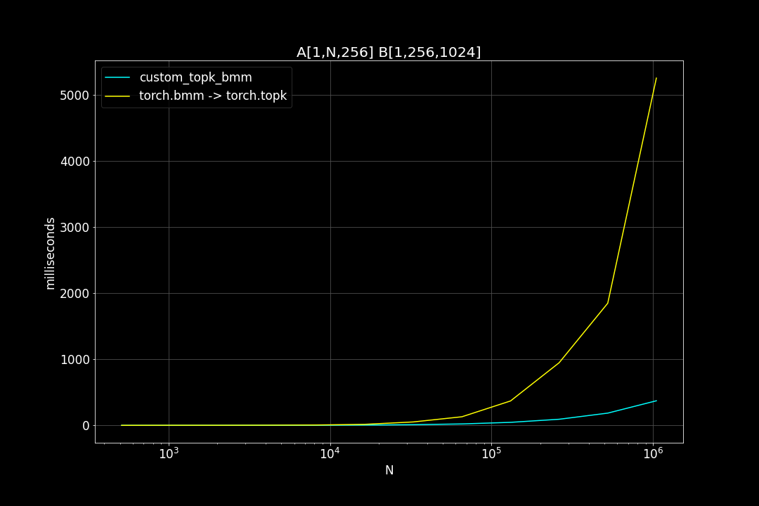
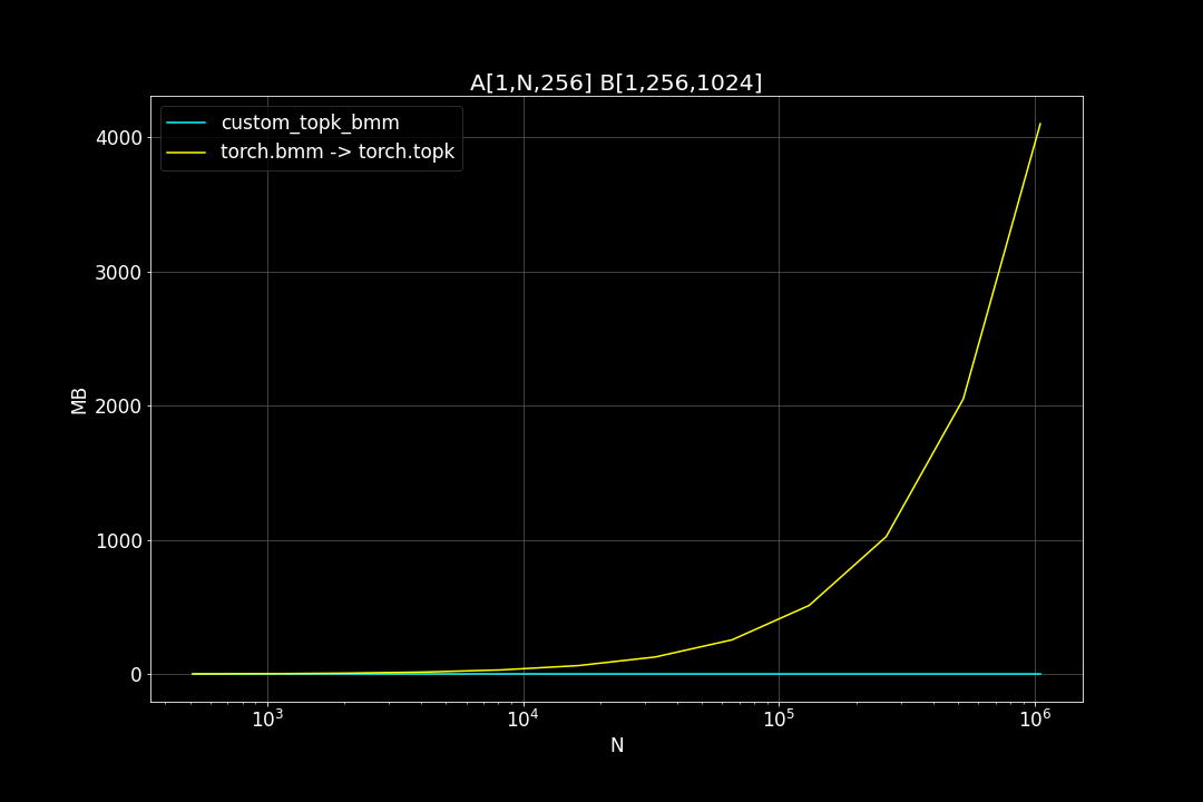
(OUTDATED) Click here to show plots
A is a (n_data x d_vector) matrix, B is a (d_vector x n_query) matrix , n_data is the number of data points, n_query is the number of query vectors, d_vector is the vector dimensionality.
n_query = 1024, d_vector = 64, varying n_data:
Runtime (ms)
Peak Memory Usage (MB)

n_query = 1024, d_vector = 256, varying n_data:
Runtime (ms)
Maximum Memory Footprint (MB)
n_query = 1024, d_vector = 1024, varying n_data:
Runtime (ms)
Peak Memory Usage (MB)
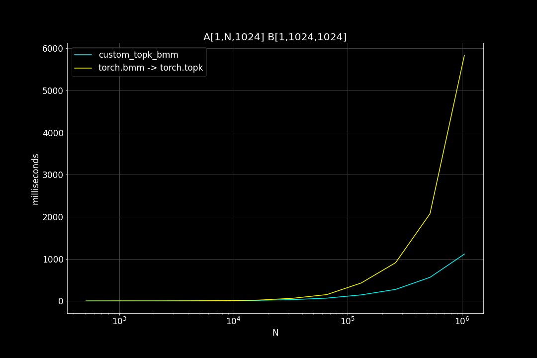

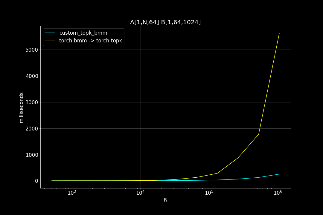
We can see that TopkBMM kernel is extremely fast! it’s up to 10x faster than the naive “bruteforce search” when n_data is close to a million and d_vector = 64. To be honest I totally wasn’t expecting this. And this is not the end! We can further improve its speed by switching to half type (float16 or bfloat16), it’s also possible to use tensor cores of more recent nvidia GPUs to accelerate the matrix multiplication. But that’s for future, I still haven’t figured out how to use WMMA with CuPy.
One limitation is that TopkBMM can search up to 128 nearest neighbors at most. In order to search for more than 128 neighbors, we can do this iteratively. For example, first search the top 128 neighbors, then 128 ~ 256, then 256 ~ 384, and so on.
UPDATE
The TopkBMM kernel that I originally wrote was a prototype that only works under specific assumptions, such as:
- both n_data and n_query are divisible by 128
- K in topk is 128
- topk operation is performed on the first dimention of the output matrix c
- the underlying memory storage is in row major order (C order) for both a and b.
I wrote a more complete version of TopkBMM later, that works for both C order and Fortan order input matrices, and supports any K value that is under 128, and supports topk on both first and second dimentions of c. However, when benchmarking the TopkBMM kernel when dim == 1, I found out that the torch.topk was performing much faster than before. It turns out that torch.topk is faster on the contiguous dimention compared to other non-contiguous dimentions.
c = torch.randn(M, N)
topk_value, topk_index = c.topk(dim=1, k=k) # this is fast
topk_value, topk_index = c.topk(dim=0, k=k) # this is a lot slower
This is why when I benchmarked my original TopkBMM kernel, it was up to 10 times faster than torch.topk(torch.bmm(a, b)), it’s not because my kernel was that much faster, it’s because the torch.topk was not used correctly. There is a trick to speed up torch.topk when performed on a non-contiguous dimention:
\((A \cdot B)^T = B^T \cdot A^T\)
c = torch.bmm(b.transpose(-1, -2), a.transpose(-1, -2))
topk_value, topk_index = c.topk(dim=-1, k=k)
TODO: add new benchmark results.
Masked BMM
Masked BMM means “hiding” some portion of the output of BMM using a binary mask. One use case of this operation is the self-attention layer of GPT style language models. After computing dot product of queries and keys, we fill the upper triangular half of the output matrix with -∞. Here is how it’s usually done in pytorch:
# shape of keys: [batch_size, M, K]
# shape of values: [batch_size, K, N]
# shape of mask: [M, N]
dot = torch.bmm(keys, queries)
dot.masked_fill_(mask = mask, value = float("-inf") )
Mask pattern

If we could fuse masked_fill into the matmul kernel, we not only can get rid of computation of masked_fill, but the BMM kernel itself can take advantage of the sparcity given by the mask (by not computing the masked part), reducing computation even further.
The matmul kernel splits the output matrix into a grid of 128 x 128 submatrices, each submatrix is assigned to a thread block. Each thread block consists of 256 threads, and each thread computes an 8 x 8 block of the 128 x 128 submatrix.
First we need to do some preprocessing. We need 3 different levels of mask: block mask, thread mask and element mask. Block mask indicates which thread blocks should be ignored, and the same goes for thread mask and element mask.
M, N = mask.shape
assert M % 128 == 0
assert N % 128 == 0

element_mask = mask
thread_mask = mask.view( M//8, 8, N//8, 8)
thread_mask = thread_mask.sum(dim=1).sum(dim=3)
block_mask = mask.view(M//128, 128, N//128, 128)
block_mask = block_mask.sum(dim=1).sum(dim=3)
For simplicity, here we assume both M and N are divisible by 128.
We input all 3 masks to the MBMM kernel:
extern "C"
__global__ void mbmm_nn(
  const float* __restrict__ A,
  const float* __restrict__ B,
  float* __restrict__ C,
  const uint8_t* __restrict__ BlockMask,   //
  const uint8_t* __restrict__ ThreadMask,  //
  const uint8_t* __restrict__ ElementMask, //
  int M, int N, int K
){
  ...
}
At the very start of the kernel, all threads within a thread block will read the block mask value, if it is 0, all threads within that thread block will exit. (No memory store/loads, no arithmetic ops.)
int bN = (N + 128 - 1) / 128;
uint8_t block_mask = BlockMask[(blockIdx.y)*bN + (blockIdx.x)];
if (block_mask == 0){
  return;
}
Each thread in the grid also reads a unique thread mask value:
int vx = threadIdx.x % 16;
int vy = threadIdx.x / 16;
uint8_t thread_mask = ThreadMask[(blockIdx.y*16 + vy)*tN + (blockIdx.x*16 + vx) ];
If it’s 0, then that thread skips thread_matmul.
// main loop
for (int i=0; i<nItr; i++)
{
  ...

  if (thread_mask != 0){
    thread_matmul(aSM, bSM, cCache, vx, vy);
  }
  __syncthreads();
}
However, all threads still participate in loading matrix A and B from global memory.
At the end of the kernel, before storing cached results to C, each thread will check its thread mask value once again, if it’s between 0 and 64, that thread will mask the cached result using element mask.
if (0 < thread_mask < 64){
  mask_cCache(cCache, ElementMask, gStartx, gStarty, vx, vy, bid, M, N);
}
write_c(cCache, C, gStartx, gStarty, vx, vy, bid, M, N);
This is kind of similar to the idea of Block Sparse. The difference is instead of designing a new kernel, we’re taking advantage of the grid-threadblock-thread hierarchy of BMM kernel to introduce sparcity. This works very well when there are lots of (128 x 128) masked blocks in our mask.
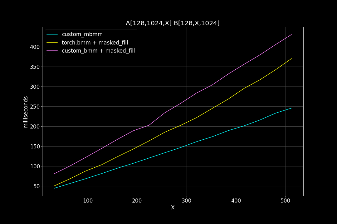
Now let’s see how the new MBMM kernel performs compared to the original BMM + masked_fill and torch.bmm (cuBLAS) + masked_fill:
Click to show plots
1. batch size = 128, M = N = 1024, varying K
Runtime (ms):
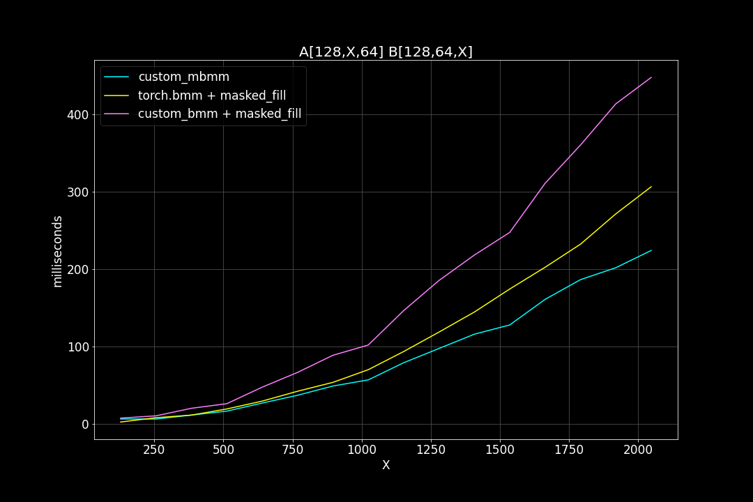
2. batch size = 128, K = 64, varying M, N (M = N)
Runtime (ms):
3. M = N = 1024, K = 128, varying batch size
Runtime (ms):
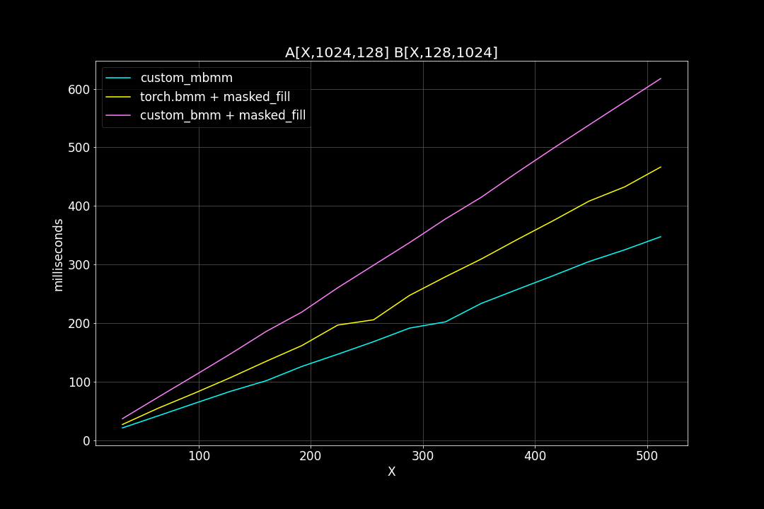
We can see that, the new MBMM kernel has roughly 2 times the speed of the original BMM kernel + masked_fill, and 1.2 ~ 1.4 times the speed of torch.bmm + masked_fill.
Selective BMM
to be continued…