In my previous post, I discussed the similarity-based bigram model (Dagan et al., 1998) and showed its performance against other classic ngram smoothing techniques. Although the original similarity-based bigram model had less perplexity than the Katz backoff model, it didn’t fare as well as the interpolated Kneser-Ney model on both Penn-tree bank (PTB) and Wikitext103 datasets. In this blog post, I’ll introduce a new similarity-based bigram model with better performance.

A Refined Model

This new similarity-based model, based on Dagan et al’s work, includes several evidence-based modifications. The first notable change is eliminating backoff. The final probability estimate, represented as \(\hat{P}\), now stems directly from \(P_r\), which is a mixture of a raw similarity-based estimate, \(P_{SIM}\), and a complementary model \(P_c\). The weightage of each part in the final estimate is controlled by an interpolation parameter, \(\lambda\). This is a variable value between \([0, 1]\), and can be set using a hyperparameter search procedure, like grid search.

\[\hat{P}(w_2 \mid w_1) = P_{r}(w_2 \mid w_1) = \gamma P_c(w_2 \mid w_1) + (1 - \gamma)P_{SIM}(w_2 \mid w_1)\]

In the original model, \(P_{SIM}\) was calculated by averaging maximum likelihood estimates of the next word probability for each word in \(S(w_1)\). But in this new model, similar words in \(S(w_1)\) are used to estimate bigram counts, and then \(P_{SIM}\) is derived by normalizing these estimates.

\[\tilde{C}(w_1, w_2) = \sum_{w_1^ \prime \in S(w_1)} C(w_1^ \prime, w_2) \dfrac{ W(w_1^ \prime, w_1) }{ \sum_{w_1'' \in S(w_1)}W(w_1'', w_1) }\] \[P_{SIM}(w_2 \mid w_1) = \dfrac {\tilde{C}(w_1, w_2)} {\sum_{w_1^ \prime \in S(w_1)} \tilde{C}(w_1^\prime, w_2)}\]

\(W(w_1^ \prime, w_1)\) stands for the adjusted similarity score. In this model, we use cosine similarity as the similarity measure, given its effectiveness in distributional semantics.

\[D(w_1, w_1 ^ \prime) = \dfrac { \vec{v}_{w_1} \cdot \vec{v}_{w_1 ^ \prime} } { \| \vec{v}_{w_1} \| \| \vec{v}_{w_1 ^ \prime} \| }\]

Cosine similarity scores are then adjusted with parameter \(\beta\) and raised to the power of e.

\[W(w_1, w_1 ^ \prime) = e^{ \beta D(w_1, w_1 ^ \prime )}\]

It’s interesting to mention that the exponential function paired with the normalization of similarity scores during \(\tilde{C}\) calculation, is essentially the same as the softmax function with temperature:

\[\dfrac{ e^{ \beta W(w_1, w_1^ \prime) } }{ \sum_{w_1^ \prime\prime \in S(w_1)} e^{ \beta W(w_1, w_1'' ) } }\]

\(\vec{v}_{w_1}\) represents the distributional vector representation of \(w_1\). We’ll explore two possible distributional methods:

Log of Laplace (LOG)

\[(\vec{v}_a)_i = \log( C(a, V_i) + 1)\]

Positive pointwise mutual information (PPMI)

\[(\vec{v}_a)_i = \max\left(0, \log \dfrac{ \tilde{P}(a, V_i) }{ \tilde{P}(a) \tilde{P}(V_i) } \right)\]

where

\[\tilde{P}(a, V_i) = \dfrac{C(a, V_i) + r}{ C(*) + r |V|^2 }\]

and

\[\tilde{P}(a) = \dfrac{C(a) + r |V|}{ C(*) + r |V|^2 }\]

Here, \((\vec{v}_a)_i\) denotes the i’th element of the vector \(\vec{v}_a\), and similarly \(V_i\) refers to the i’th word in the vocabulary. $C(*)$ is the total number of words in the dataset, and $r$ is a free parameter that’s added to all of the bigram counts to avoid 0 probabilities.

The complementary model, $P_c$, can be picked from the existing n-gram methods. We will consider the unigram model, Katz backoff model, and Kneser-Ney bigram and unigram models as possible choices for the complementary model.

Experiments

Before we dive into our proposed method, let’s first review the performance of other baseline models:

model	PPL (PTB)	PPL (Wikitext2)	PPL (Wikitext103)
Laplace	335.5	182.5	86.2
Good-Turing	152.1	101.4	80.5
Katz	138.8	97.6	80.6
Kneser-Ney(\(d\)=0.75)	118.9	88.1	77.6
Dagan et al.(\(\gamma\)=0.06, \(\beta\)=10, \(k\)=50, \(t\)=10)	128.4	97.1	80.5

Influence of $k$ and the distributional method

We keep \(\gamma=0.06\), \(\beta=10.0\), \(t=0.1\), \(r=1.0\), and \(P_c\) as a unigram model, and analyze the impact of varying distributional methods and \(k\) on the model’s performance:

method	\(k\)	PPL (PTB)	PPL (Wikitext2)	PPL (Wikitext103)
LOG	40	126.7	93.9	108.0
LOG	80	123.6	93.2	114.2
LOG	160	123.6	92.9	118.6
LOG	320	119.9	93.3	122.7
PPMI	40	129.6	93.9	84.0
PPMI	80	127.4	93.7	85.6
PPMI	160	125.5	93.6	87.0
PPMI	320	124.1	93.7	88.4

When we pick a unigram model as the complementary model, we see that the perplexity of our modified model on smaller datasets like Wikitext2 or PTB is generally lower than the original model. Larger \(k\) values tend to yield better results. It’s also quite noticeable that LOG outperforms PPMI when the dataset is smaller. However, for the larger dataset (Wikitext103), the trends change. Firstly, LOG seems to perform much worse than PPMI, and larger \(k\) values don’t necessarily lead to lower perplexities. Next, let’s take a closer look at the effect of \(k\) on model perplexity on Wikitext103 dataset:

Influence of \(k\) on Wikitext103

\(k\)	method	PPL (Wikitext103)
1	PPMI	78.9
2	PPMI	79.7
3	PPMI	80.3
5	PPMI	81.1
10	PPMI	82.4
20	PPMI	84.0
30	PPMI	85.0

The testset perplexity seems to hit its lowest when \(k=1\). Meaning, when the set of similar words \(S(w_1)\) only contains one word, which is \(w_1\) itself. In this case, \(P_{SIM}(w_2 \mid w_1)\) would simply equal \(P_{MLE}(w_2 \mid w_1)\). This implies that the similarity-based model is only worsening the performance. This observation suggests that the benefit of similarity-based generalization decreases as the dataset size grows larger. To verify this, we’ll investigate the effect of trainset size on test set perplexity. We’ll use different fractions of all the bigrams in the Wikitext103 trainset to train the model and see how \(k\) impacts the model performance:

We notice a qualitative difference between using 0.1% to 1% and 10% to 100% of the trainset. Higher values of \(k\) lead to lower perplexities when the fraction of the trainset used is below 1%, but when it’s above 10%, the perplexity is at its lowest when \(k=1\). This aligns with our earlier hypothesis that similarity-based generalization is only helpful when the dataset is smaller. Could this be a hyperparameter issue, particularly the parameter \(r\), which is added to the count of all bigrams before calculating the similarities?

Influence of \(r\) on different fractions of Wikitext103

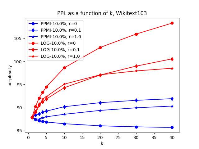
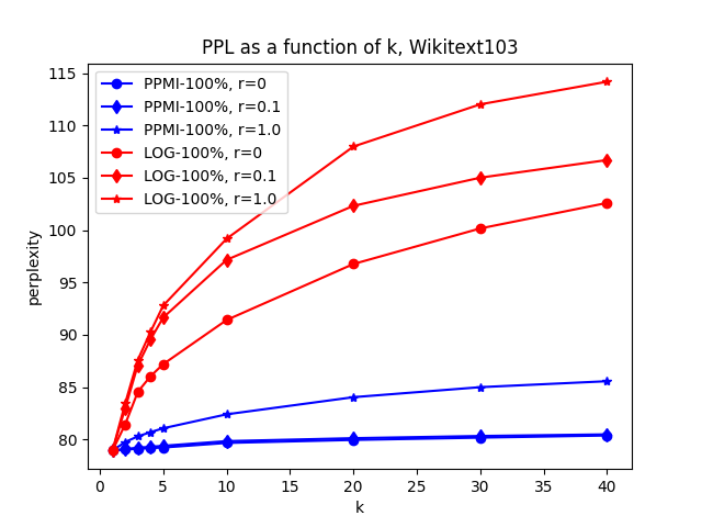
Examining the plot, it’s clear that the choice of \(r\) directly affects the model’s perplexity. When we only use 1% of the trainset (~1M words), LOG with \(r=1.0\) is the clear winner. When we use 10% of the trainset (~10M words), and set \(r=0\) with PPMI, we notice the model performance improving as k grows, indicating the effectiveness of the similarity-based model. However, when the entire trainset is used to train the model, the similarity-based model still fails to improve performance, as the testset perplexity still increases as we increase k from 1. However, when \(r=0\), the rate of perplexity increase is much slower than \(r=1\).

In conclusion, the similarity-based estimation seems to be most helpful when the model is trained on a smaller trainset (\(\leq 10 M\) words), however, on larger corpora such as Wikitext103, it may negatively affect model perplexity. But this conclusion may only apply to this specific version of similarity-based models.

Next, we will see how the choice of \(\gamma\) and \(P_c\) impacts model perplexity.

effect of \(P_c\) and \(\gamma\) on PTB and Wikitext2

This time, we fix \(t=0.1\), \(r=1.0\), \(k=40\) and use LOG as the method for measuring distributional similarity.

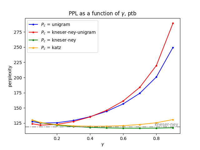
As we can observe, using the Kneser-Ney bigram model as the complementary model seems to deliver the best results, which isn’t surprising given the reputation of the Kneser-Ney model among N-gram models. Importantly, when \(\gamma=0.7\), the mix of the Kneser-Ney model and similarity-based model outperforms the Kneser-Ney model alone, with a 2% and 1.5% drop in testset perplexity on PTB and Wikitext2, respectively. Next, let’s see if we can maximize this by increasing the value of \(k\):

effect of \(k\) on PTB and Wikitext2

n addition to the fixed parameters used in the previous experiment, we also set \(\gamma=0.7\) and use the Kneser-Ney model with \(d=0.75\) as \(P_c\).

k	PPL (PTB)	PPL (Wikitext2)
40	116.48 (-2.0%)	86.84 (-1.5%)
80	115.79 (-2.6%)	86.58 (-1.8%)
160	115.24 (-3.2%)	86.41 (-1.9%)
320	114.89 (-3.5%)	86.37 (-2.0%)
640	114.85 (-3.5%)	86.44 (-1.9%)

Further increasing \(k\) indeed results in lower perplexities, however, we notice a clear trend of diminishing returns. \(k=320\) seems to be the threshold beyond which further increases don’t provide meaningful improvements.

Up until this point, we have kept most of the other parameters fixed. From the multitude of experiments I conducted that are not included in this article, I’ve observed that models are generally very insensitive to the value of \(t\), as long as it’s not very high. Finally, let’s see if altering \(\beta\) provides any improvement.

effect of \(\beta\) on PTB and Wikitext2

We still use the same fixed parameters used in the previous experiment, while changing the value of \(\beta\):

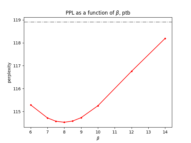
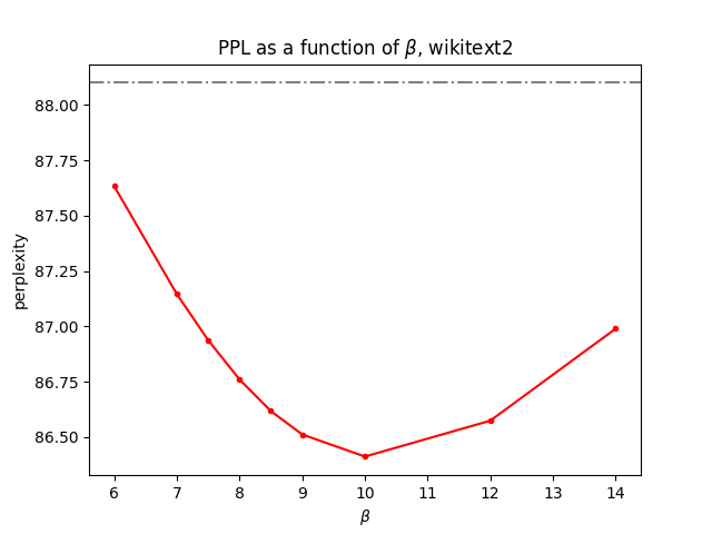
It seems that the optimal \(\beta\) varies depending on the dataset. For PTB, a \(\beta\) value of 8.0 appears to yield the best results. On the other hand, for Wikitext2, a \(\beta\) value of 10.0 seems to be the most effective.

Wrapping Up

To sum up, our experiments have shown that the similarity-based model is particularly effective with smaller datasets. While it can’t quite match the Kneser-Ney model on its own, it performs better when combined with Kneser-Ney model. However, when we tested our similarity-based approach on larger datasets, like the Wikitext103, it didn’t really contribute to reducing the test set perplexity. This might suggest that this similarity-based approach is better suited to smaller datasets. But it’s important to keep in mind that this limitation might only apply to our current model, and there could be other, more sophisticated similarity-based models out there that can efficiently incorporate the advantages of models like the Kneser-Ney model.

Up next, we will extend the formulation of our similarity-based bigram model to N-grams of any order, starting with trigram models. As we do this, we’ll start to consider compositionality, a key feature of natural language.